Markov Chains
A Markov chain refers to a sequence (or "chain") of discrete events, generated according to a fixed set of probabilistic rules. The most important property of these rules is that they can only refer to the current state of the system, and cannot depend on the past states of the system. Markov chains have numerous applications in physics, mathematics, and computing. In statistical mechanics, for instance, Markov chains are used to describe the random sequence of micro-states visited by a system undergoing thermal fluctuations.
Contents[hide] |
The simplest Markov chain: the coin-flipping game
Game description
Before giving the general description of a Markov chain, let us study a few specific examples of simple Markov chains. One of the simplest is a "coin-flip" game. Suppose we have a coin which can be in one of two "states": heads (H) or tails (T). At each step, we flip the coin, producing a new state which is H or T with equal probability. In this way, we generate a sequence like "HTTHTHTTHH..." If we run the game again, we would generate another different sequence, like "HTTTTHHTTH..." Each of these sequences is a Markov chain.
This process can be visualized using a "state diagram":
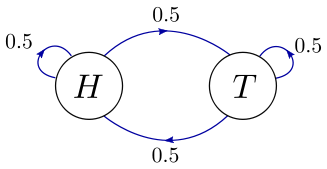
Here, the two circles represent the two possible states of the system, "H" and "T", at any step in the coin-flip game. The arrows indicate the possible states that the system could transition into, during the next step of the game. Attached to each arrow is a number giving the probability of that transition. For example, if we are in the state "H", there are two possible states we could transition into during the next step: "T" (with probability 0.5), or "H" (with probability 0.5). By conservation of probability, the transition probabilities coming out of each state must sum up to one.
Next, suppose the coin-flipping game is unfair. The coin might be heavier on one side, so that it is overall more likely to land on H than T. It might also be slightly more likely to land on the same face that it was flipped from (real coins actually do behave this way). The resulting state diagram can look like this:
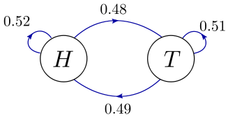
Notice that the individual transition probabilities are no longer 0.5, reflecting the aforementioned unfair effects. However, the transition probabilities coming out of each state still sum to 1 (0.52+0.48 coming out of "H", and 0.51+0.49 coming out of "T").
State probabilities
If we play the above unfair game many times, H and T will tend to
occur with slightly different probabilities, not exactly equal to 0.5.
At a given step, let  denote the probability to be in state H, and
  the probability to be in state T. Let
  denote the transition probability for going from H to T, during the
next step; and similarly for the other three possible transitions.
According to Bayes' rule, we can write the probability to get H on the next step as
denote the transition probability for going from H to T, during the
next step; and similarly for the other three possible transitions.
According to Bayes' rule, we can write the probability to get H on the next step as

Similarly, the probability to get T on the next step is

We can combine these into a single matrix equation:
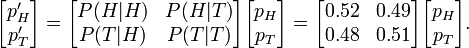
The matrix of transition probabilities is called the transition matrix. At the beginning of the game, we can specify the coin state to be (say) H, so that  and
and  .
If we multiply the vector of state probabilities by the transition
matrix, that gives the state probabilities for the next step.
Multiplying by the transition matrix
.
If we multiply the vector of state probabilities by the transition
matrix, that gives the state probabilities for the next step.
Multiplying by the transition matrix  times gives the state probabilities after steps.
After a large number of steps, the states probabilities might
converge to a "stationary" distribution, such that they no longer change
significantly on subsequent steps. Let these stationary probabilities
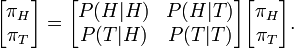
be denoted by  . According to the above equation for transition probabilities, the stationary probabilities must satisfy
This system of linear equations can be solved by brute force (we'll discuss a more systematic approach later). The result is

Plugging in the numerical values for the transition probabilities, we end up with  .
.
General description
Markov processes
More generally, suppose we have a system possessing a discrete set of states, which can be labeled by an integer  A Markov process
is a set of probabilistic rules that tell us how to choose a new state
of the system, based on the system's current state. If the system is
currently in state
A Markov process
is a set of probabilistic rules that tell us how to choose a new state
of the system, based on the system's current state. If the system is
currently in state  , then the probability of choosing state
  on the next step is denoted by
  . We call this the "transition probability" from state to state . By repeatedly applying the Markov process, we move the system through a random sequence of states,
 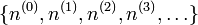 , where
  denotes the state on step
  . This kind of random sequence is called a Markov chain.
There is an important constraint on the transition probabilities of the Markov process. Because the system must transition to some state on each step,
Next, we introduce the idea of state probabilities. Suppose we look at the ensemble of all possible Markov chains which can be generated by a given Markov process. Let  denote the probabilities for the various states,
  , on step . Given these, what are the probabilities for the various states on step
  ? According to Bayes' theorem, we can write
  as a sum over conditional probabilities:
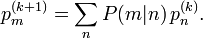
This has the form of a matrix equation:
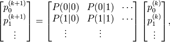
where the matrix on the right-hand side is called the transition matrix. Each element of this matrix is a real number between 0 and 1; furthermore, because of the aforementioned conservation of transition probabilities, each column of the matrix sums to 1. In mathematics, matrices of this type are called "left stochastic matrices".
Stationary distribution
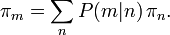
A stationary distribution is a set of state probabilities 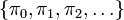 , such that passing through one step of the Markov process leaves the probabilities unchanged:
By looking at the equivalent matrix equation, we see the vector ![[\pi_0; \pi_1; \pi_2; \dots]](PH4505_files/ed8d1094ced068c420f86993ec5d7e36.png) must be an eigenvector of the transition matrix, with eigenvalue 1. It turns out that there is a mathematical theorem (the Perron–Frobenius theorem)
which states every left stochastic matrix has an eigenvector of this
sort. Hence, every Markov process possesses a stationary distribution.
Stationary distributions are the main reasons we are interested in
Markov processes. In physics, we are often interested in using Markov
processes to model thermodynamic systems, such that a stationary
distribution represents the distribution of thermodynamic micro-states
under thermal equilibrium. (We'll see an example
in the next section.) Knowing the stationary distribution, we can
figure out all the thermodynamic properties of the system, such as its
average energy.
must be an eigenvector of the transition matrix, with eigenvalue 1. It turns out that there is a mathematical theorem (the Perron–Frobenius theorem)
which states every left stochastic matrix has an eigenvector of this
sort. Hence, every Markov process possesses a stationary distribution.
Stationary distributions are the main reasons we are interested in
Markov processes. In physics, we are often interested in using Markov
processes to model thermodynamic systems, such that a stationary
distribution represents the distribution of thermodynamic micro-states
under thermal equilibrium. (We'll see an example
in the next section.) Knowing the stationary distribution, we can
figure out all the thermodynamic properties of the system, such as its
average energy.
In principle, one way to figure out the stationary distribution is to construct the transition matrix, solve the eigenvalue problem, and pick out the eigenvector with eigenvalue 1. The trouble is that we are often interested in systems where the number of possible states is huge—in some cases, larger than the number of atoms in the universe! In such cases, it is not possible to explicitly generate the transition matrix, let alone solve the eigenvalue problem.
We now come upon a happy and important fact: for a huge class of Markov processes, the distribution of states within a sufficiently long Markov chain will converge to the stationary distribution. Hence, in order to find out about the stationary distribution, we simply need to generate a long Markov chain, and study its statistical properties.
The Ehrenfest model
Model description
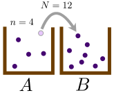
The coin-flipping game is a "two-state" Markov chain. For physics applications, we're often interested in Markov chains where the number of possible states is huge (e.g. thermodynamic microstates). The Ehrenfest model is a nice and simple example which illustrates many of the properties of such Markov chains. This model was introduced by the husband-and-wife physicist team of Paul and Tatyana Ehrenfest in 1907, in order to study the physics of diffusion.
Suppose we have two boxes, labeled A and B, and a total of  distinguishable particles to distribute between the two boxes. At a given point in time, let there be particles in box A, and hence
  particles in box B. Now, we repeatedly apply the following procedure:
- Randomly choose one of the particles (with equal probability).
- With probability
 , move the chosen particle from whichever box it happens to be into the other box. Otherwise (with probability
  ), leave the particle in its current box.
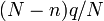
If there are particles in box A, then we have probability  of choosing a particle in box A, followed by a probability of
to move that particle into box B. Following similar logic for all the
other possibilities, we arrive at three possible outcomes:
of choosing a particle in box A, followed by a probability of
to move that particle into box B. Following similar logic for all the
other possibilities, we arrive at three possible outcomes:
- Move a particle from A to B: probability

- Move a particle from B to A: probability
- Leave the system unchanged: probability
You can check that (i) the probabilities sum up to 1, and (ii) this summary holds true for the end-cases  and
and  .
.
Markov chain description
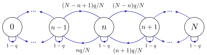
We can label the states of the system using an integer 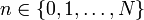 , corresponding to the number of particles in box A. There are
  possible states, and the state diagram is as follows:
Suppose we start out in state  ,
by putting all the particles in box A. As we repeatedly apply the
Ehrenfest procedure, the system goes through a sequence of states,
,
by putting all the particles in box A. As we repeatedly apply the
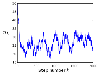
Ehrenfest procedure, the system goes through a sequence of states, 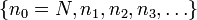 , which can be described as a Markov chain. Plotting the state
  versus the step number , we see a random trajectory like the one below:
 and
and  .
.Notice that the system moves rapidly away from its initial state,  , and settles into a behavior where it fluctuates around the mid-point state
  .
Let us look for the stationary distribution, in which the probability
of being in each state is unchanged on subsequent steps. Let
.
Let us look for the stationary distribution, in which the probability
of being in each state is unchanged on subsequent steps. Let  denote the stationary probability for being in state . According to Bayes' rule, this probability distribution needs to satisfy

We can figure out
using two different methods. The first method is to use our knowledge
of statistical mechanics. In the stationary distribution, each
individual particle should have an equal chance of being in box A or box
B. There are  possible box assignments, each of which is energetically equivalent and
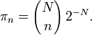
hence have equal probabilities. Hence, the probability of finding particles in box A is the number of ways of picking particles, which is
possible box assignments, each of which is energetically equivalent and
hence have equal probabilities. Hence, the probability of finding particles in box A is the number of ways of picking particles, which is  , divided by the number of possible box assignments. This gives
Substituting into the Bayes' rule formula, we can verify that this distribution is indeed stationary. Note that turns out to be independent of (the probability of transferring a chosen particle to the other box). Intuitively,
governs how "quickly" we are transferring particles from one box to the
other. Therefore, it should affect how quickly the system reaches its
stationary or "equilibrium" behavior, but not the stationary
distribution itself.
Detailed balance
There is another way to figure out , which doesn't rely on guessing the answer in one shot. Suppose we pick a pair of neighboring states, and  , and assume that the rate at which the
  transition occurs is the same as the rate at which the opposite transition, , occurs. Such a condition is not guaranteed to hold, but if it holds for every pair of states, then the probability distribution is necessarily stationary. This situation is called detailed balance. In terms of the state probabilities and transition probabilities, detailed balance requires

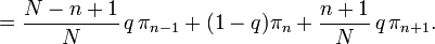
for this Markov chain. Plugging in the transition probabilities, we obtain the recursion relation
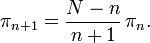
What's convenient about this recursion relation is that it only involves and  , unlike the Bayes' rule relation which also included
  . By induction, we can now easily show that
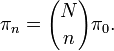
By conservation of probability,  , we can show that
  . This leads to
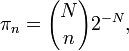
which is the result that we'd previously guessed using purely statistical arguments.
For more complicated Markov chains, it may not be possible to guess the stationary distribution; in such cases, the detailed balance argument is often the best approach. Note, however, that the detailed balance condition is not guaranteed to occur. There are some Markov chains which do not obey detailed balance, so we always need to verify that the detailed balance condition's result is self-consistent (i.e., that it can indeed be obeyed for every pair of states).
Computational physics notes | Prev: Discrete Fourier transform Next: Markov chain Monte Carlo method
