Finite-Difference Equations

One of the most common tasks in scientific computing is finding solutions to differential equations, because most physical theories are formulated using differential equations. In classical mechanics, for example, a mechanical system is described by a second-order differential equation in time (Newton's second law); and in classical electromagnetism, the electromagnetic fields are described by first-order partial differential equations in space and time (Maxwell's equations).

In order to describe continuous functions (and the differential equations that act on them), computational schemes usually adopt the strategy of discretization. Consider a general mathematical function of one real variable, $\psi(x)$ , where the domain of the input is $\mathbb{R}$ , or some finite interval. In principle, in order to fully specify the function, we have to enumerate its values for all possible inputs $x$ ; but since $x$ can vary continuously, the set is uncountably infinite, so such an enumeration is impossible on a digital computer with finite discrete memory. What we can do, instead, is to enumerate the function's values at a finite and discrete set of points,

: $\{x_n \;|\; n = 0, 1, 2, \dots, N-1\}.$

We define the values at these points as

: $\psi_n \equiv \psi(x_n).$

If $x_n$ is appropriately chosen, the set of values $\{\psi_n\}$ ought to describe $\psi(x)$ quite accurately. One reason for this is that physical theories typically involve differential equations of low order (e.g., first, second, or third order, rather than, say, order 1,000,000). Hence, if the discretization points are sufficiently finely-spaced, the value of the function, and all its higher-order derivatives, will vary only slightly between discretization points.

As we shall see, discretization converts differential equations into discrete systems of equations, called finite-difference equations. These can then be solved using the standard methods of numerical linear algebra.

Derivatives

Suppose we have discretized a function of one variable, obtaining a set of $\psi_n \equiv \psi(x_n)$ as described above. For simplicity, we assume that the discretization points are evenly-spaced and arranged in increasing order (this is the simplest and most common discretization scheme). The spacing between points is defined as

: $h \equiv x_{n+1} - x_n.$

Let us discuss how the first and higher-order derivatives of $\psi(x)$ can be represented under discretization.

First derivative

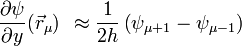
The most straightforward representation of the first derivative is the forward-difference formula:

: $\psi'(x_n) \approx \frac{\psi_{n+1} - \psi_n}{h}$

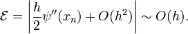
This is inspired by the usual definition of the derivative of a function, and approaches the true derivative as $h \rightarrow 0$ . However, it is not a very good approximation. To see why, let's analyze the error in the formula, which is defined as the absolute value of the difference between the formula and the exact value of the derivative:

: $\mathcal{E} = \left|\psi'(x_n) - \frac{\psi_{n+1} - \psi_n}{h}\right|$

We can expand $\psi_{n+1}$ in a Taylor series around $x_n$ :

: $\psi_{n+1} = \psi_n + h\, \psi'(x_n) + \frac{h^2}{2}\psi''(x_n) + \frac{h^3}{6}\psi'''(x_n) + O(h^4)$

Plugging this into the error formula, we find that the error decreases linearly with the spacing:

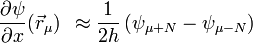
: $\mathcal{E} = \left| \frac{h}{2}\psi''(x_n) + O(h^2)\right| \sim O(h).$

There is a better alternative, called the mid-point formula. This approximates the first derivative by sampling the points to the left and right of the desired position:

: $\psi'(x_n) \approx \frac{\psi_{n+1} - \psi_{n-1}}{2h}.$

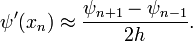
To see why this is better, let us write down the Taylor series for $\psi_{n\pm1}$ :

: $\psi_{n+1} = \psi_n \,+\, h\, \psi'(x_n) \,+\, \frac{h^2}{2}\psi''(x_n) \,+\, \frac{h^3}{6}\psi'''(x_n) \,+\, \frac{h^4}{24}\psi''''(x_n) + O(h^5)$
: $\psi_{n-1} = \psi_n \,-\, h\, \psi'(x_n) \,+\, \frac{h^2}{2}\psi''(x_n) \,-\, \frac{h^3}{6}\psi'''(x_n) \,+\, \frac{h^4}{24}\psi''''(x_n) \,+\, O(h^5)$

Note that the two series have the same terms involving even powers of $h$ , whereas the terms involving odd powers of $h$ have opposite signs. Hence, if we subtract the second series from the first, the result is

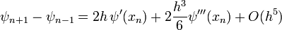
: $\psi_{n+1} - \psi_{n-1} = 2 h\, \psi'(x_n) + 2 \frac{h^3}{6}\psi'''(x_n) + O(h^5)$

Because the $O(h^2)$ terms are equal in the two series, they cancel out under subtraction, and only the $O(h^3)$ and higher terms survive. After re-arranging the above equation, we get

: $\psi'(x_n) = \frac{\psi_{n+1} - \psi_{n-1}}{2 h} + O(h^2).$

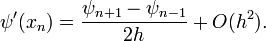
Hence, the error of the mid-point formula scales as $O(h^2)$ , which is a good improvement over the $O(h)$ error of the forward-difference formula. What's especially nice is that the mid-point formula requires the same number of arithmetic operations to calculate as the forward-difference formula, so this is a free lunch!

It is possible to come up with better approximation formulas for the first derivative by including terms involving $\psi_{n\pm 2}$ etc., with the goal of canceling the $O(h^3)$ or higher terms in the Taylor series. For most practical purposes, however, the mid-point rule is sufficient.

Second derivative

The discretization of the second derivative is easy to figure out too. We again write down the Taylor series for $\psi_{n\pm1}$ :

: $\psi_{n+1} = \psi_n \,+\, h\, \psi'(x_n) \,+\, \frac{h^2}{2}\psi''(x_n) \,+\, \frac{h^3}{6}\psi'''(x_n) \,+\, \frac{h^4}{24}\psi''''(x_n) \,+\, O(h^5)$
: $\psi_{n-1} = \psi_n \,-\, h\, \psi'(x_n) \,+\, \frac{h^2}{2}\psi''(x_n) \,-\, \frac{h^3}{6}\psi'''(x_n) \,+\, \frac{h^4}{24}\psi''''(x_n) \,+\, O(h^5)$

When we add the two series together, the terms involving odd powers of $h$ cancel, and the result is

: $\psi_{n+1} + \psi_{n-1} = 2\psi_n + h^2 \psi''(x_n) + \frac{h^4}{12}\psi''''(x_n) + O(h^5).$

A minor rearrangement of the equation then gives

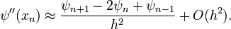
: $\psi''(x_n) \approx \frac{\psi_{n+1} - 2\psi_n + \psi_{n-1}}{h^2} + O(h^2).$

This is called the three-point rule for the second derivative, because it involves the value of the function at the three points $x_{n+1}$ , $x_{n}$ , and $x_{n-1}$ .

Discretizing partial differential equations

With discretized derivatives, differential equations can be formulated as discrete systems of equations. We will discuss this using a specific example: the discretization of the time-independent Schrödinger wave equation in 1D.

Deriving a finite-difference equation

The 1D time-independent Schrödinger wave equation is the second-order ordinary differential equation

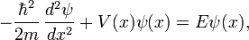
: $-\frac{\hbar^2}{2m} \, \frac{d^2\psi}{dx^2} + V(x) \psi(x) = E \psi(x),$

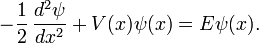
where $\hbar$ is Planck's constant divided by $2\pi$ , $m$ is the mass of the particle, $V(x)$ is the potential, $\psi(x)$ is the quantum wavefunction of an energy eigenstate of the particle, and $E$ is the corresponding energy. The differential equation is usually treated as an eigenproblem, in the sense that we are given $V(x)$ and seek to find the possible values of the eigenfunction $\psi(x)$ and the energy eigenvalue $E$ . For convenience, we will adopt units where $\hbar=m = 1$ :

: $-\frac{1}{2}\, \frac{d^2\psi}{dx^2} + V(x) \psi(x) = E \psi(x).$

To discretize this differential equation, we simply evaluate it at $x = x_n$ :

: $-\frac{1}{2}\, \psi''(x_n) + V_n \psi_n = E \psi_n,$

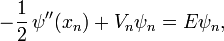
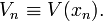
where, for conciseness, we denote

: $V_n \equiv V(x_n).$

We then replace the second derivative $\psi''(x_n)$ with a discrete approximation, specifically the three-point rule:

: $-\frac{1}{2h^2}\, \Big[\psi_{n+1} - 2\psi_n + \psi_{n-1} \Big] + V_n \psi_n = E \psi_n.$

This result is called a finite-difference equation, and it would be valid for all $n$ if the number of discretization points is infinite. However, if there is a finite number of discretization points, $\{x_0, x_1, \dots, x_{N-1}\}$ , then the finite-difference formula fails at the boundary points, $n = 0$ and $n = N-1$ , where it involves the value of the function at the "non-existent" points $x_{-1}$ and $x_N$ . We'll see how to handle this problem in the next section.

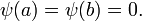
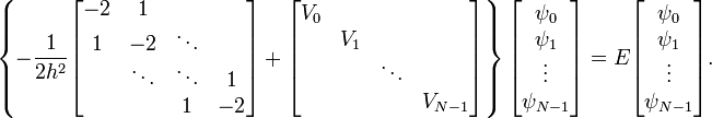
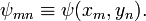
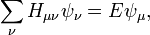
Boundaries aside, the finite-difference equation describes a matrix equation:

: $\left\{-\frac{1}{2h^2}\begin{bmatrix} \ddots & \ddots \\ \ddots & -2 & 1\\ & 1 & -2 & 1\\ & & 1 & -2 & \ddots \\ & & & \ddots & \ddots & \end{bmatrix} + \begin{bmatrix} & \ddots & \\ & & V_{n-1} & \\ & & & V_n & \\ & & & & V_{n+1} & \\ & & & & & \ddots \end{bmatrix} \right\}\begin{bmatrix}\vdots \\ \psi_{n-1} \\ \psi_n \\ \psi_{n+1} \\ \vdots\end{bmatrix} = E \begin{bmatrix}\vdots \\ \psi_{n-1} \\ \psi_n \\ \psi_{n+1} \\ \vdots\end{bmatrix}.$

The second-derivative operator is represented by a tridiagonal matrix with $-2$ in each diagonal element, and $1$ in the elements directly above and below the diagonal. The potential operator is represented by a diagonal matrix, where the elements along the diagonal are the values of the potential at each discretization point. In this way, the Schrödinger wave equation is reduced to a discrete eigenvalue problem.

Boundary conditions

We now have to figure out how to handle the boundaries. Let us suppose $\psi(x)$ is defined over a finite interval, $a \le x \le b$ . As we recall from the theory of differential equations, the solution to a differential equation is not wholly determined by the differential equation itself, but also by the boundary conditions that are imposed. Thus, we have to specify how $\psi(x)$ behaves at the end-points of the interval. We will show how this is done for a couple of the most common boundary conditions; other choices of boundary conditions can be handled using the same kind of reasoning.

Dirichlet boundary conditions

Under Dirichlet boundary conditions, the wavefunction vanishes at the boundaries:

: $\psi(a) = \psi(b) = 0.$

Physically, these boundary conditions apply if we let the potential blow up in the external regions, $x > b$ and $x < a$ , thus forcing the wavefunction to be strictly confined to the interval $a \le x \le b$ .

We have not yet stated how the discretization points $\{x_0, \dots, x_{N-1}\}$ are distributed within the interval; we will make this decision in tandem with the implementation of the boundary conditions. Consider the first discretization point, $x_0$ , wherever it is. The finite-difference equation at this point is

: $-\frac{1}{2h^2}\, \Big[\psi_{-1} - 2\psi_0 + \psi_{1} \Big] + V_0 \psi_0 = E \psi_0.$

This involves the wavefunction at $x_{-1}$ , which lies just outside our set of discretization points. But if we choose the discretization points so that $x_{-1} = a$ , then $\psi_{-1} = 0$ under Dirichlet boundary conditions, so the above finite-difference formula reduces to

: $-\frac{1}{2h^2}\, \Big[- 2\psi_0 + \psi_{1} \Big] + V_0 \psi_0 = E \psi_0.$

As for the other boundary, the finite-difference equation at $x_{N-1}$ involves $\psi_{N}$ . If we choose the discretization points so that $x_{N} = b$ , then the finite-difference formula becomes

: $-\frac{1}{2h^2}\, \Big[ \psi_{N-2} - 2\psi_{N-1} \Big] + V_{N-1} \psi_{N-1} = E \psi_{N-1}.$

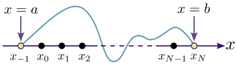
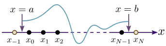
From this, we conclude that the discretization points ought to be equally spaced, with $x_0$ at a distance $h$ to the right of the left boundary $a$ and $x_{N-1}$ a distance $h$ to the left of the right boundary $b$ . This is shown in the following figure:

Fig. 1: Position of discretization points for Dirichlet boundary conditions at $x = a$ and $x = b$ .

Since there are $N$ discretization points, the interval should contain $(N+1)$ multiples of $h$ . Hence,

: $h = \frac{b - a}{N + 1} \;\; \Rightarrow \;\; x_n \,=\, a + h (n+1) \,=\, \frac{a(N-n)+b(n+1)}{N+1}.$

Having made the above choices, the matrix equation becomes

: $\left\{-\frac{1}{2h^2}\begin{bmatrix} -2 & 1 \\ 1 & -2 & \ddots \\ & \ddots & \ddots & 1 \\ & & 1 & -2\end{bmatrix} + \begin{bmatrix} V_0 \\ & V_1 \\ & & \ddots\\ & & & V_{N-1} \end{bmatrix} \right\}\begin{bmatrix}\psi_0 \\ \psi_1 \\ \vdots \\ \psi_{N-1}\end{bmatrix} = E \begin{bmatrix}\psi_0 \\ \psi_1 \\ \vdots \\ \psi_{N-1}\end{bmatrix}.$

You can check for yourself that the first and last rows of this equation are the correct finite-difference equations at the boundary points, corresponding to Dirichlet boundary conditions.

Neuman boundary conditions

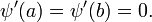
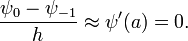
Neumann boundary conditions are another common choice of boundary conditions. They state that the first derivatives vanish at the boundaries:

: $\psi'(a) = \psi'(b) = 0.$

An example of such a boundary condition is encountered in electrostatics, where the first derivative of the electric potential goes to zero at the surface of a charged metallic surface.

We follow the same strategy as before, figuring out the discretization points in tandem with the boundary conditions. Consider again the finite-difference equation at the first discretization point:

: $-\frac{1}{2h^2}\, \Big[\psi_{-1} - 2\psi_0 + \psi_{1} \Big] + V_0 \psi_0 = E \psi_0.$

To implement the condition that first derivative vanishes at the boundary, we invoke the mid-point rule. Suppose the boundary point $x = a$ falls in between the points $x_{-1}$ and $x_0$ . Then, according to the mid-point rule,

: $\frac{\psi_0 - \psi_{-1}}{h} \approx \psi'(a) = 0.$

With this choice, therefore, we can make the replacement $\psi_{-1} = \psi_0$ in the finite-difference equation, which then becomes

: $-\frac{1}{2h^2}\, \Big[- \psi_0 + \psi_{1} \Big] + V_0 \psi_0 = E \psi_0.$

Similarly, to apply the Neumann boundary condition at $x = b$ , we let the boundary fall between $x_{N-1}$ and $x_N$ , so that the finite-difference equation becomes

: $-\frac{1}{2h^2}\, \Big[ \psi_{N-2} - \psi_{N-1} \Big] + V_{N-1} \psi_{N-1} = E \psi_{N-1}.$

The resulting distribution of discretization points is shown in the following figure:

Fig. 2: Position of discretization points for Neumann boundary conditions at $x = a$ and $x = b$ .

Unlike the Dirichlet case, the interval contains $N$ multiples of $h$ . Hence, we get a different formula for the positions of the discretization points

: $h = \frac{b - a}{N} \;\; \Rightarrow \;\; x_n \,=\, a + h \left(n+\frac{1}{2}\right) \,=\, \frac{a(N-n-\tfrac{1}{2})+b(n+\tfrac{1}{2})}{N}.$

The matrix equation is:

: $\left\{-\frac{1}{2h^2}\begin{bmatrix} -1 & 1 \\ 1 & -2 & \ddots \\ & \ddots & \ddots & \ddots \\ && \ddots & -2 & 1 \\ & & & 1 & -1\end{bmatrix} + \begin{bmatrix} V_0 \\ & V_1 \\ & & \ddots\\ & & & V_{N-1} \end{bmatrix} \right\}\begin{bmatrix}\psi_0 \\ \psi_1 \\ \vdots \\ \psi_{N-1}\end{bmatrix} = E \begin{bmatrix}\psi_0 \\ \psi_1 \\ \vdots \\ \psi_{N-1}\end{bmatrix}.$

Due to the Neumann boundary conditions and the mid-point rule, the tridiagonal matrix has $-1$ instead of $-2$ on its corner entries. Again, you can verify that the first and last rows of this matrix equation correspond to the correct finite-difference equations for the boundary points.

Higher dimensions

We can work out the finite-difference equations for higher dimensions in a similar manner. In two dimensions, for example, the wavefunction $\psi(x,y)$ is described with two indices:

: $\psi_{mn} \equiv \psi(x_m, y_n).$

The discretization of the derivatives is carried out in the same way, using the mid-point rule for first partial derivatives in each direction, and the three-point rule for the second partial derivative in each direction. Let us suppose that the discretization spacing is equal in both directions:

: $h = x_{m+1} - x_m = y_{n+1} - y_n.$

Then, for the second derivative, the Laplacian operator

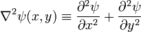
: $\nabla^2 \psi(x,y) \equiv \frac{\partial^2\psi}{\partial x^2} + \frac{\partial^2\psi}{\partial y^2}$

can be approximated by a five-point rule, which involves the value of the function at $(m,n)$ and its four nearest neighbours:

: $\nabla^2\psi(x_m,y_n) \approx \frac{\psi_{m+1,n} + \psi_{m,n+1} - 4\psi_{mn} + \psi_{m-1,n} + \psi_{m,n-1}}{h^2} + O(h^2).$

For instance, the finite-difference equations for the 2D Schrödinger wave equation is

: $-\frac{1}{2h^2}\, \Big[\psi_{m+1,n} + \psi_{m,n+1} - 4\psi_{mn} + \psi_{m-1,n} + \psi_{m,n-1} \Big] + V_{mn} \psi_{mn} = E \psi_{mn}.$

Matrix reshaping

Higher-dimensional differential equations introduce one annoying complication: in order to convert between the finite-difference equation and the matrix equation, the indices have to be re-organized. For instance, the matrix form of the 2D Schrödinger wave equation should have the form

: $\sum_{\nu} H_{\mu\nu} \psi_\nu = E \psi_\mu,$

where the wavefunctions are organized into a 1D array labeled by a "point index" $\mu$ . Each point index corresponds to a pair of "grid indices", $(m,n)$ , representing spatial coordinates on a 2D grid. We have to be careful not to mix up the two types of indices.

We will adopt the following conversion scheme between point indices and grid indices:

: $\mu(m,n) = m N + n,\quad \mathrm{where}\; m \in \{ 0, \dots, M-1\}, \;\; n \in \{ 0, \dots, N-1\}.$

One good thing about this conversion scheme is that Scipy provides a reshape function which can convert a 2D array with grid indices $(m,n)$ into a 1D array with the point index $\mu$ :

>>> a = array([[0,1,2],[3,4,5],[6,7,8]])
>>> a
array([[0, 1, 2],
       [3, 4, 5],
       [6, 7, 8]])
>>> b = reshape(a, (9))     # Reshape a into a 1D array of size 9
>>> b
array([0, 1, 2, 3, 4, 5, 6, 7, 8])

The reshape function can also convert a 1D back into the 2D array, in the right order:

>>> c = reshape(b, (3,3))   # Reshape b into a 2D array of size 3x3
>>> c
array([[0, 1, 2],
       [3, 4, 5],
       [6, 7, 8]])

Under point indices, the discretized derivatives take the following forms:

: $\frac{\partial \psi}{\partial x}(\vec{r}_\mu)\;\, \approx \frac{1}{2h} \left(\psi_{\mu+N} - \psi_{\mu-N}\right)$; $\frac{\partial \psi}{\partial y}(\vec{r}_\mu)\;\, \approx \frac{1}{2h} \left(\psi_{\mu+1} - \psi_{\mu-1}\right)$; $\nabla^2\psi(\vec{r}_\mu) \approx \frac{1}{h^2} \left(\psi_{\mu+N} + \psi_{\mu+1} - 4\psi_{\mu} + \psi_{\mu-N} + \psi_{\mu-1}\right).$

The role of boundary conditions is left as an exercise. There are now two sets of boundaries, at $m \in \{0,M-1\}$ and $n \in \{0, N-1\}$ . By examining the finite-difference equations along each boundary, we can (i) assign the right discretization coordinates and (ii) modify the finite-difference matrix elements to fit the boundary conditions. The details are slightly tedious to work out, but the logic is essentially the same as in the previously-discussed 1D cases.